2 Data ingestion patterns
This chapter covers
- Understanding data ingestion and its responsibilities
- Handling large datasets in memory by consuming smaller datasets in batches (the batching pattern)
- Preprocessing extremely large datasets as smaller chunks on multiple machines (the sharding pattern)
- Fetching and re-accessing the same dataset for multiple training rounds (the caching pattern)
Chapter 1 discussed the growing scale of modern machine learning applications such as larger datasets and heavier traffic for model serving. It also talked about the complexity and challenges of building distributed systems–distributed systems for machine learning applications in particular. We learned that a distributed machine learning system is usually a pipeline of many components, such as data ingestion, model training, serving, and monitoring, and that some established patterns are available for designing each component to handle the scale and complexity of real-world machine learning applications.
All data analysts and scientists should have some level of exposure to data ingestion, either hands-on experience in building a data ingestion component or simply using a dataset from the engineering team or customer. Designing a good data ingestion component is nontrivial and requires understanding the characteristics of the dataset we want to use for building a machine learning model. Fortunately, we can follow established patterns to build that model on a reliable and efficient foundation.
This chapter explores some of the challenges involved in the data ingestion process and introduces a few established patterns adopted heavily in industries. In section 2.3, we will use the batching pattern in cases where we want to handle and prepare large datasets for model training, either when the machine learning framework we are using cannot handle large datasets or requires domain expertise in the underlying implementation of the framework. In section 2.4, we will learn how to apply the sharding pattern to split extremely large datasets into multiple data shards spread among multiple worker machines; then we speed up the training process as we add worker machines that are responsible for model training on each data shard independently. Section 2.5 introduces the caching pattern, which could greatly speed up the data ingestion process when a previously used dataset is re-accessed and processed for multi-epoch model training.
2.1 What is data ingestion?
Let’s assume that we have a dataset at hand, and we would like to build a machine learning system that builds a machine learning model from it. What is the first thing we should think about? The answer is quite intuitive: first, we should get a better understanding of the dataset. Where did the dataset come from, and how was it collected? Are the source and the size of the dataset changing over time? What are the infrastructure requirements for handling the dataset? We should ask these types of questions first. We should also consider different perspectives that might affect the process of handling the dataset before we start building a distributed machine learning system. We will walk through these questions and considerations in the examples in the remaining sections of this chapter and learn how to address some of the problems we may encounter by using different established patterns.
Data ingestion is the process that monitors the data source, consumes the data all at once (nonstreaming) or in a streaming fashion, and performs preprocessing to prepare for the training process of machine learning models. In short, streaming data ingestion often requires long-running processes to monitor the changes in data sources; nonstreaming data ingestion happens in the form of offline batch jobs that process datasets on demand. Additionally, the data grows over time in streaming data ingestion, whereas the size of the dataset is fixed in nonstreaming data ingestion. Table 2.1 summarizes the differences.
| Streaming data ingestion | Nonstreaming data Ingestion | |
|---|---|---|
| Dataset size | Increases over time | Fixed size |
| Infrastructure requirements | Long-running processes to monitor the changes in data source | Offline batch jobs to process datasets on demand |
The remaining sections of this chapter focus on data ingestion patterns from a nonstreaming perspective, but they can be applied to streaming data ingestion as well.
Data ingestion is the first step and an inevitable step in a machine learning pipeline, as shown in figure 2.1. Without a properly ingested dataset, the rest of the processes in a machine learning pipeline would not be able to proceed.
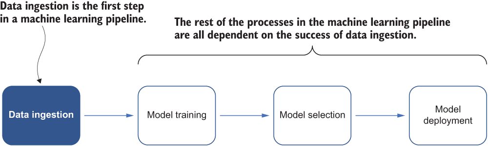
The next section introduces the Fashion-MNIST dataset, which I use to illustrate the patterns in the remaining sections of this chapter. I focus on building patterns around data ingestion in distributed machine learning applications, which are distinct from data ingestion that happens on local machines or laptops. Data ingestion in distributed machine learning applications is often more complex and requires careful design to handle large-scale datasets or datasets that are growing rapidly.
2.2 The Fashion-MNIST dataset
The MNIST dataset by LeCun et al. (http://yann.lecun.com/exdb/mnist/) is one of the most widely used datasets for image classification. It contains 60,000 training images and 10,000 testing images extracted from images of handwritten digits; it is used widely in the machine learning research community as a benchmark dataset to validate state-of-art algorithms and machine learning models. Figure 2.2 shows some example images of handwritten digits, with each row representing images of a particular handwritten digit.
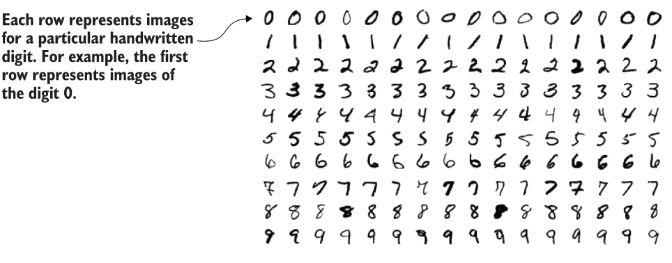
Despite wide adoption in the community, researchers have found this dataset to be unsuitable for distinguishing between stronger models and weaker ones; many simple models nowadays can achieve good classification accuracy over 95%. As a result, the MNIST dataset now serves as more a sanity check than a benchmark.
Note The creators of the MNIST dataset kept a list of the machine learning methods tested on the dataset. In the original paper, “Gradient-Based Learning Applied to Document Recognition,” published in 1998 on the MNIST dataset (http://yann.lecun.com/exdb/publis/index.html#lecun-98), LeCun et al. stated that they used a support-vector machine model to get an error rate of 0.8%. A similar but extended dataset called EMNIST was published in 2017. EMNIST contains 240,000 training images and 40,000 testing images of handwritten digits and characters.
Instead of using MNIST in several examples throughout this book, I will focus on a quantitatively similar but relatively more complex dataset: the Fashion-MNIST dataset, which was released in 2017 (https://github.com/zalandoresearch/fashion-mnist). Fashion-MNIST is a dataset of Zalando’s article images consisting of a training set of 60,000 examples and a test set of 10,000 examples. Each example is a 28 × 28 grayscale image associated with a label from ten classes. The Fashion-MNIST dataset is designed to serve as a direct drop-in replacement for the original MNIST dataset for benchmarking machine learning algorithms. It uses the same image size and structure for training and testing splits.
Figure 2.3 shows the collection of images for all 10 classes (T-shirt/top, trouser, pullover, dress, coat, sandal, shirt, sneaker, bag, and ankle boot) from Fashion-MNIST. Each class takes up three rows of the screenshot.
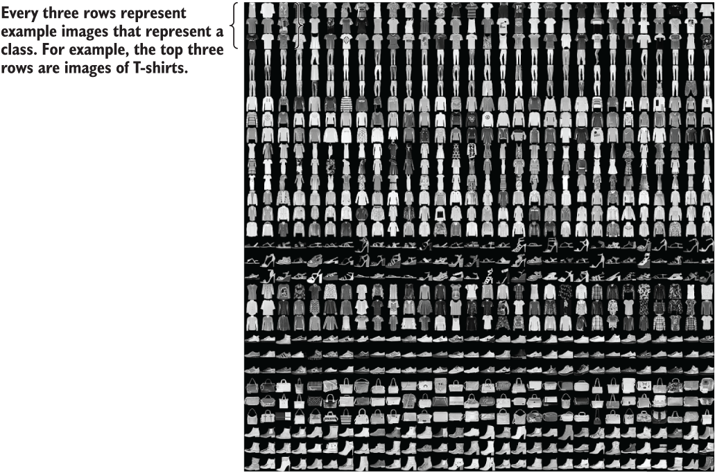
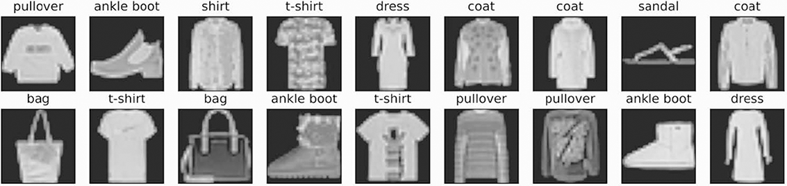
Figure 2.4 provides a closer look at the first few example images in the training set, together with their corresponding text labels. Next, I discuss the scenario for the case study.
Assume that we’ve downloaded the Fashion-MNIST dataset. The compressed version should only take 30 MB on disk. Even though the dataset is small, it’s trivial to load the downloaded dataset into memory at one time by using available implementations. If we’re using a machine learning framework like TensorFlow, for example, we can download and load the entire Fashion-MNIST dataset into memory with a couple of lines of Python code, as shown in the following listing.
Listing 2.1 Loading the Fashion-MNIST dataset into memory with TensorFlow
> import tensorflow as tf ❶
>
> train, test = tf.keras.datasets.fashion_mnist.load_data() ❷
32768/29515 [=================================] - 0s 0us/step
26427392/26421880 [==============================] - 0s 0us/step
8192/5148 [===============================================] - 0s 0us/step
4423680/4422102 [==============================] - 0s 0us/step
❶ Loads the TensorFlow library
❷ Downloads the Fashion-MNIST dataset and then loads it into memory
Alternatively, if the dataset is already in memory–in the form of NumPy (https://numpy.org) arrays, for example–we can load the dataset from an in-memory array representation into formats that the machine learning framework accepts, such as tf.Tensor objects, which can easily be used for model training later. The following listing shows an example.
Listing 2.2 Loading the Fashion-MNIST dataset from memory into TensorFlow
> from tensorflow.data import Dataset
>
> images, labels = train ❶
> images = images/255 ❷
>
> dataset = Dataset.from_tensor_slices((images, labels)) ❸
> dataset ❹
<TensorSliceDataset shapes: ((28, 28), ()), types: (tf.float64, tf.uint8)>
❶ Splits the training dataset object into images and labels
❷ Normalizes the images
❸ Loads in-memory array representation into a tf.data.Dataset object that will make it easier to use for training in TensorFlow
❹ Inspects the dataset’s information, such as shapes and data types
2.3 Batching pattern
Now that we know what the Fashion-MNIST dataset looks like, let’s examine a potential problem we might face in a real-world scenario.
2.3.1 The problem: Performing expensive operations for Fashion MNIST dataset with limited memory
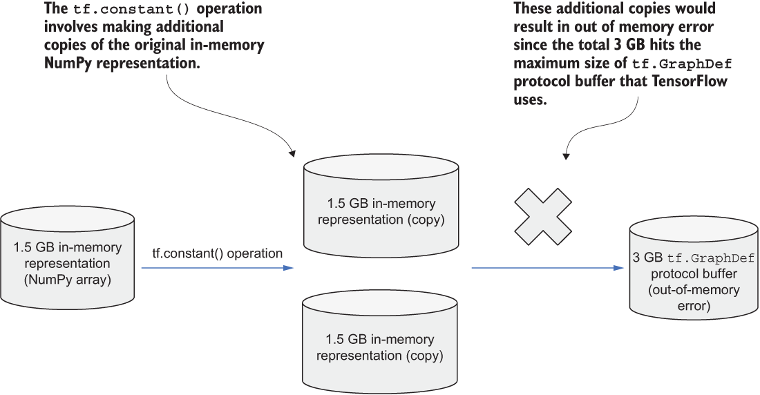
Even though it’s easy to load a small dataset like Fashion-MNIST into memory to prepare for model training, in real-world machine learning applications, this process can be challenging. The code snippet in listing 2.1, for example, can be used to load the Fashion-MNIST into memory to prepare for model training in TensorFlow; it embeds the features and labels arrays in our TensorFlow graph as tf.constant() operations. This process works well for a small dataset, but it wastes memory because the contents of the NumPy array will be copied multiple times and can run into the 2 GB limit for the tf.GraphDef protocol buffer that TensorFlow uses. In real-world applications, the datasets are much larger, especially in distributed machine learning systems in which datasets grow over time.
Figure 2.5 shows a 1.5-GB in-memory NumPy array representation that will be copied two times with a tf.constant() operation. This operation would result in an out-of-memory error because the total 3 GB exceeds the maximum size of the tf.GraphDef protocol buffer that TensorFlow uses.
tf.GraphDef protocol bufferProblems like this one happen often in different machine learning or data loading frameworks. Users may not be using the specific framework in an optimal way, or the framework may not be able to handle larger datasets.
In addition, even for small datasets like Fashion-MNIST, we may perform additional computations before feeding the dataset into the model, which is common in tasks that require additional transformations and cleaning. For computer vision tasks, images often need to be resized, normalized, or converted to grayscale, or they may require even more complex mathematical operations, such as convolution operations. These operations may require a lot of additional memory space allocation, but we may not have many computational resources available after we load the entire dataset into memory.
2.3.2 The solution
Consider the first problem mentioned in section 2.2. We’d like to use TensorFlow’s from_tensor_slices() API to load the Fashion-MNIST dataset from an in-memory NumPy array representation to a tf.Dataset object that TensorFlow’s model training program can use. Because the contents of the NumPy array will be copied multiple times, however, we can run into the 2 GB limit for the tf.GraphDef protocol buffer. As a result, we cannot load larger datasets that go beyond this limit.
It’s not uncommon to see problems like this one for specific frameworks like TensorFlow. In this case, the solution is simple because we are not making the best use of TensorFlow. Other APIs allow us to load large datasets without loading the entire dataset into in-memory representation first.
TensorFlow’s I/O library, for example, is a collection of filesystems and file formats that are not available in TensorFlow’s built-in support. We can load datasets like MNIST from a URL to access the dataset files that are passed directly to the tfio.IODataset.from_mnist() API call, as shown in the following listing. This ability is due to the inherent support that TensorFlow (https://github.com/tensorflow/io) I/O library provides for the HTTP filesystem, eliminating the need to download and save datasets in a local directory.
Listing 2.3 Loading the MNIST dataset with TensorFlow I/O
> import tensorflow_io as tfio ❶
>
> d_train = tfio.IODataset.from_mnist( ❷
'http:/ /yann.lecun.com/exdb/mnist/train-images-idx3-ubyte.gz',
'http:/ /yann.lecun.com/exdb/mnist/train-labels-idx1-ubyte.gz')
❶ Loads the TensorFlow I/O library
❷ Loads the MNIST dataset from a URL to access dataset files directly without downloading via HTTP filesystem support
For larger datasets that might be stored in distributed file systems or databases, some APIs can load them without having to download everything at one time, which could cause memory- or disk-related problems. For demonstration purposes, without going into too many details here, the following listing shows how to load a dataset from a PostgreSQL database (https://www.postgresql.org). (You’ll need to set up your own PostgreSQL database and provide the required environment variables to run this example.)
Listing 2.4 Loading a dataset from the PostgreSQL database
> import os ❶
> import tensorflow_io as tfio ❷
>
> endpoint="postgresql://{}:{}@{}?port={}&dbname={}".format( ❸
os.environ['TFIO_DEMO_DATABASE_USER'],
os.environ['TFIO_DEMO_DATABASE_PASS'],
os.environ['TFIO_DEMO_DATABASE_HOST'],
os.environ['TFIO_DEMO_DATABASE_PORT'],
os.environ['TFIO_DEMO_DATABASE_NAME'],
)
>
> dataset = tfio.experimental.IODataset.from_sql( ❹
query="SELECT co, pt08s1 FROM AirQualityUCI;",
endpoint=endpoint)
> print(dataset.element_spec) ❺
{
'co': TensorSpec(shape=(), dtype=tf.float32, name=None),
'pt08s1': TensorSpec(shape=(), dtype=tf.int32, name=None)
}
❶ Loads Python’s built-in OS library for loading environment variables related to the PostgreSQL database
❷ Loads the TensorFlow I/O library
❸ Constructs the endpoint for accessing the PostgreSQL database
❹ Selects two columns from the AirQualityUCI table in the database and instantiates a tf.data.Dataset object
❺ Inspects the specification of the dataset, such as the shape and data type of each column
Now let’s go back to our scenario. In this case, assume that TensorFlow does not provide APIs like TensorFlow I/O that can deal with large datasets. Given that we don’t have too much free memory, we should not load the entire Fashion-MNIST dataset into memory directly. Let’s assume that the mathematical operations we would like to perform on the dataset can be performed on subsets of the entire dataset. Then we can divide the dataset into smaller subsets (mini-batches), load each mini-batch of example images, perform expensive mathematical operations on each batch, and use only one mini-batch of images in each model training iteration.
If the first mini-batch consists of the 19 example images in figure 2.4, we can perform convolution or other heavy mathematical operations on those images first and then send the transformed images to the machine learning model for model training. We repeat the same process for the remaining mini-batches while continuing model training in the meantime.
Because we’ve divided the dataset into many small subsets or mini-batches, we avoid potential out-of-memory problems when performing the heavy mathematical operations necessary for achieving an accurate classification model. Then we can handle even larger datasets by reducing the size of the mini-batches. This approach is called batching. In data ingestion, batching involves grouping data records from the entire dataset into batches that will be used to train the machine learning model sequentially.
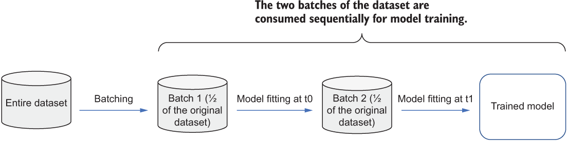
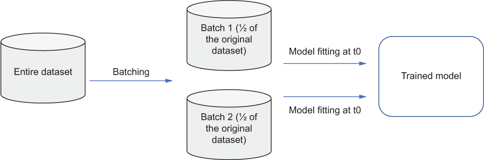
If we have a dataset with 100 records, we can take 50 of the 100 records to form a batch and then train the model using this batch of records. We repeat this batching and model training process for the remaining records. In other words, we make two batches in total; each batch consists of 50 records, and the model we are training consumes the batches one by one. Figure 2.6 illustrates the process of dividing the original dataset into two batches. The first batch gets consumed to train the model at time t0, and the second batch gets consumed at time t1. As a result, we don’t have to load the entire dataset into memory at one time; instead, we are consuming the dataset sequentially, batch by batch.
This batching pattern can be summarized as the pseudocode in the following listing, where we continuously try to read the next batch from the dataset and train the model, using the batches until no more are left.
Listing 2.5 Pseudocode for batching
batch = read_next_batch(dataset) ❶
while batch is not None:
    model.train(batch) ❷
    batch = read_next_batch(dataset) ❸
❶ Reads the next batch in the dataset
❷ Trains the model with this batch
❸ Reads the next batch after training the current batch
We can apply the batching pattern when we want to handle and prepare large datasets for model training. When the framework we are using can handle only in-memory datasets, we can process small batches of the entire large datasets to ensure that each batch can be handled within limited memory. In addition, if a dataset is divided into batches, we can perform heavy computations on each batch sequentially without requiring a huge amount of computational resources. We’ll apply this pattern in section 9.1.2.
2.3.3 Discussion
Other considerations need to be taken into account when performing batching. This approach is feasible only if the mathematical operations or algorithms we are performing can be done on subsets of the entire dataset in a streaming fashion. If an algorithm requires knowledge of the entire dataset, such as the sum of a particular feature over the entire dataset, batching would no longer be a feasible approach, as it’s not possible to obtain this information over a subset of the entire dataset.
In addition, machine learning researchers and practitioners often try different machine learning models on the Fashion-MNIST dataset to get a better-performing, more accurate model. If an algorithm would like to see at least 10 examples for each class to initialize some of its model parameters, for example, batching is not an appropriate approach. There is no guarantee that every mini-batch contains at least 10 examples from each class, especially when batch sizes are small. In an extreme case, the batch size would be 10, and it would be rare to see at least one image from each class in all batches.
Another thing to keep in mind is that the batch size of a machine learning model, especially for deep learning models, depends strongly on allocation of resources, making it particularly difficult to decide in advance in shared-resource environments. Also, the allocation of resources that a machine learning job can use efficiently depends not only on the structure of the model being trained but also on the batch size. This codependency between the resources and the batch size creates a complex web of considerations that a machine learning practitioner must make to configure their job for efficient execution and resource use.
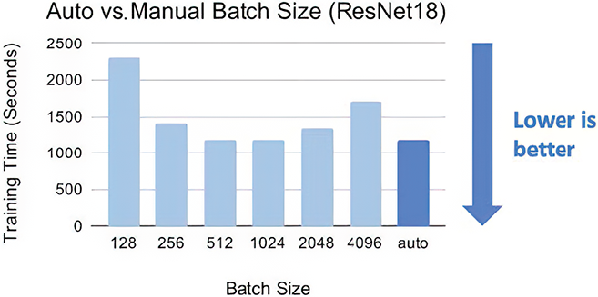
Fortunately, algorithms and frameworks are available that eliminate manual tuning of batch size. AdaptDL (https://github.com/petuum/adaptdl), for example, offers automatic batch-size scaling, enabling efficient distributed training without requiring any effort to tune the batch size manually. It measures the system performance and gradient noise scale during training and adaptively selects the most efficient batch size. Figure 2.7 compares the effects of automatically and manually tuned batch sizes on the overall training time of the ResNet18 model (https://arxiv.org/abs/1512.03385).
The batching pattern provides a great way to extract subsets of the entire dataset so that we can feed the batches sequentially for model training. For extremely large datasets that may not fit in a single machine, we’ll need other techniques. The next section introduces a new pattern in that addresses the challenges.
2.3.4 Exercises
Are we training the model using the batches in parallel or sequentially?
If the machine learning framework we are using does not handle large datasets, can we use the batching pattern?
If a machine learning model requires knowing the mean of a feature of the entire dataset, can we still use the batching pattern?
2.4 Sharding pattern: Splitting extremely large datasets among multiple machines
Section 2.3 introduced the Fashion-MNIST dataset, the compressed version of which takes only 30 MB on disk. Even though it is trivial to load the whole dataset into memory at one time, it’s challenging to load larger datasets for model training.
The batching pattern covered in section 2.3 addresses the problem by grouping data records from the entire dataset into batches that will be used to train the machine learning model sequentially. We can apply the batching pattern when we want to handle and prepare large datasets for model training, either when the framework we are using cannot handle large datasets or when the underlying implementation of the framework requires domain expertise.
Suppose that we have a much larger dataset at hand. This dataset is about 1,000 times bigger than the Fashion-MNIST dataset. In other words, the compressed version of it takes 30 MB × 1,000 = 30 GB on disk, and it’s about 50 GB when it’s decompressed. This new dataset has 60,000 × 1,000 = 60,000,000 training examples.
We’ll try to use this larger dataset to train our machine learning model to classify images into classes in the expanded Fashion-MNIST dataset (T-shirts, bags, and so on). For now, I won’t address the detailed architecture of the machine learning model (chapter 3); instead, I’ll focus on its data ingestion component. Assume that we are allowed to use three machines for any potential speed-ups.
Given our experience, because the dataset is large, we could try applying the batching pattern first, dividing the entire dataset into batches small enough to load into memory for model training. Let’s assume that our laptop has enough resources to store the entire 50 GB decompressed dataset on disk. We divide the dataset into 10 small batches (5 GB each). With this batching approach, we can handle large datasets as long as our laptop can store the large datasets and divide them into batches.
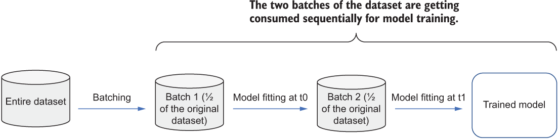
Next, we start the model training process by using the batches of data. In section 2.3, we trained the model sequentially. In other words, one batch was completely consumed by the machine learning model before the next batch was consumed. In figure 2.8, the second batch is consumed at time t1 by model fitting only after the first batch has been completely consumed by the model at time t0. t0 and t1 represent two consecutive time points in this process.
2.4.1 The problem
Unfortunately, this sequential process of consuming data can be slow. If each 5 GB batch of data takes about 1 hour to complete for the specific model we are training, it would take 10 hours to finish the model training process on the entire dataset. In other words, the batching approach may work well if we have enough time to train the model sequentially, batch by batch. In real-world applications, however, there’s always demand for more efficient model training, which will be affected by the time spent ingesting batches of data.
2.4.2 The solution
Now that we understand the slowness of training the model sequentially by using the batching pattern alone, what can we do to speed up the data ingestion part, which will greatly affect the model training process? The major problem is that we need to train the model sequentially, batch by batch. Can we prepare multiple batches and then send them to the machine learning model for consumption at the same time? Figure 2.9 shows that the dataset gets divided into two batches, with each batch being consumed to train the model at the same time. This approach does not work yet, as we cannot keep the entire dataset (two batches) in memory at the same time, but it is close to the solution.
Let’s assume that we have multiple worker machines, each of which contains a copy of the machine learning model. Each copy can consume one batch of the original dataset; hence, the worker machines can consume multiple batches independently. Figure 2.10 shows an architecture diagram of multiple worker machines; each consumes batches independently to train the copy of the model located on it.
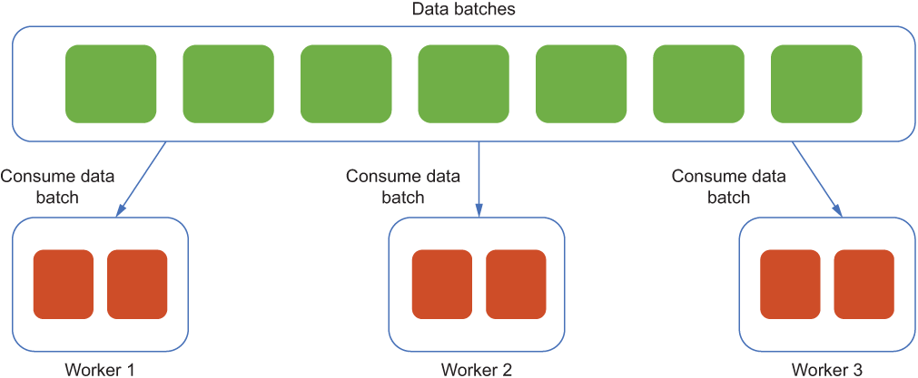
You may wonder how multiple model copies would work if they consumed multiple different batches independently and where we would obtain the final machine learning model from these model copies. These are great questions. Rest assured that I will go through how the model training process works in chapter 3. For now, assume that we have patterns that allow multiple worker machines to consume multiple batches of datasets independently. These patterns will greatly speed up the model training process, which was slowed down due to the nature of sequential model training.
Note We will be using a pattern called the collection communication pattern in chapter 3 to train models with multiple model copies located on multiple worker machines. The collective communication pattern, for example, will be responsible for communicating updates of gradient calculations among worker machines and keeping the model copies in sync.
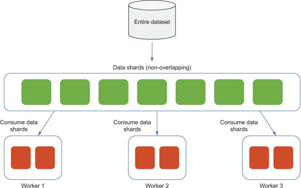
How would we produce the batches used by those worker machines? In our scenario, the dataset has 60 million training examples, and three worker machines are available. It’s simple to split the dataset into multiple non-overlapping subsets and then send each to the three worker machines, as shown in figure 2.11. The process of breaking large datasets into smaller chunks spread across multiple machines is called sharding, and the smaller data chunks are called data shards. Figure 2.11 shows the original dataset being sharded into multiple non-overlapping data shards and then consumed by multiple worker machines.
Note Although I am introducing sharding here, the concept isn’t new; it’s often used in distributed databases. Sharding in distributed databases is extremely useful for solving scaling challenges such as providing high availability of the databases, increasing throughput, and reducing query response time.
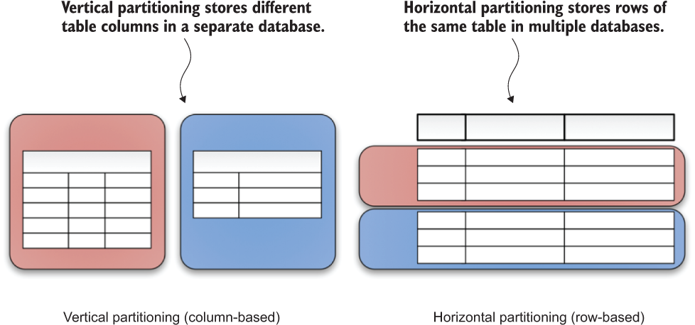
A shard is essentially a horizontal data partition that contains a subset of the entire dataset, and sharding is also referred to as horizontal partitioning. The distinction between horizontal and vertical comes from the traditional tabular view of a database. A database can be split vertically–storing different table columns in a separate database–or horizontally–storing rows of the same table in multiple databases. Figure 2.12 compares vertical partitioning and horizontal partitioning. Note that for vertical partitioning, we split the database into columns. Some of the columns may be empty, which is why we see only three of the five rows in the partition on the right side of the figure.
This sharding pattern can be summarized in the pseudocode in listing 2.6, where, first, we create data shards from one of the worker machines (in this case, worker machine with rank 0) and then send it to all other worker machines. Next, on each worker machine, we continuously try to read the next shard locally that will be used to train the model until no more shards are left locally.
Listing 2.6 Pseudocode for sharding
if get_worker_rank() == 0: ❶
    create_and_send_shards(dataset) ❶
shard = read_next_shard_locally() ❷
while shard is not None:
    model.train(shard) ❸
    shard = read_next_shard_locally() ❹
❶ Creates and sends shards to all other worker machines from the worker machine with rank 0
❷ Reads the next shard available locally in this worker machine
❸ Trains the model using the shard we just read from the worker machine locally
❹ Reads the next shard once we are done training with the current shard
With the help of the sharding pattern, we can split extremely large datasets into multiple data shards that can be spread among multiple worker machines, and then each of the worker machines is responsible for consuming individual data shards independently. As a result, we have just avoided the slowness of sequential model training due to the batching pattern. Sometimes it’s also useful to shard large datasets into subsets of different sizes so that each shard can run different computational workloads depending on the amount of computational resource available in each worker machine. We’ll apply this pattern in section 9.1.2.
2.4.3 Discussion
We have successfully used the sharding pattern to split an extremely large dataset into multiple data shards that spread among multiple worker machines and then sped up the training process as we add additional worker machines that are responsible for model training on each of the data shards independently. This is great, and with this approach, we can train machine learning models on extremely large datasets.
Now here comes the question: What if the dataset is growing continuously and we need to incorporate the new data that just arrived into the model training process? In this case, we’ll have to reshard every once in a while if the dataset has been updated to rebalance each data shard to make sure they are split relatively evenly among the different worker machines.
In section 2.3.2, we simply divided the dataset into two non-overlapping shards, but unfortunately in real-world systems, this manual approach is not ideal and may not work at all. One of the most significant challenges with manual sharding is uneven shard allocation. The disproportionate distribution of data could cause shards to become unbalanced, with some overloaded while others remain relatively empty. This imbalance could cause unexpected hanging of the model training process that involves multiple worker machines, which we’ll talk about further in the next chapter. Figure 2.13 is an example where the original dataset gets sharded into multiple imbalanced data shards and then consumed by multiple worker machines.
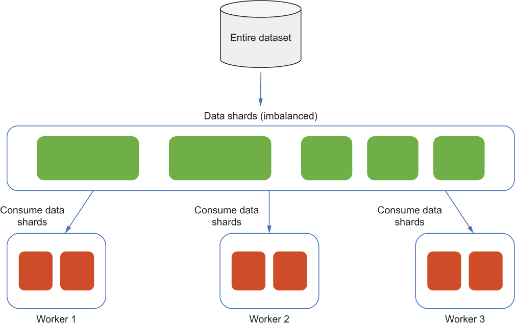
It’s best to avoid having too much data in one individual shard, which could lead to slowdowns and machine crashes. This problem could also happen when we force the dataset to be spread across too few shards. This approach is acceptable in development and testing environments but not ideal in production.
In addition, when manual sharding is used every time we see an update in the growing dataset, the operational process is nontrivial. Now we will have to perform backups for multiple worker machines, and we must carefully coordinate data migration and schema changes to ensure that all shards have the same schema copy.
To address that problem, we can apply autosharding based on algorithms instead of manually sharding datasets. Hash sharding, shown in figure 2.14, takes the key value of a data shard, which generates a hash value. Then the generated hash value is used to determine where a subset of the dataset should be located. With a uniform hashing algorithm, the hash function can distribute data evenly across different machines, reducing the problems mentioned earlier. In addition, data with shard keys that are close to one another are unlikely to be placed in the same shard.
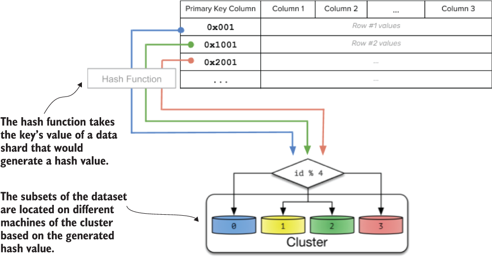
The sharding pattern works by splitting extremely large datasets into multiple data shards spread among multiple worker machines; then each of the worker machines is responsible for consuming individual data shards independently. With this approach, we can avoid the slowness of sequential model training due to the batching pattern. Both the batching and sharding patterns work well for the model training process; eventually, the dataset will be iterated thoroughly. Some machine learning algorithms, however, require multiple scans of the dataset, which means that we might perform batching and sharding twice. The next section introduces a pattern to speed up this process.
2.4.4 Exercises
Does the sharding pattern introduced in this section use horizontal partitioning or vertical partitioning?
Where does the model read each shard from?
Is there any alternative to manual sharding?
2.5 Caching pattern
Let’s recap the patterns we’ve learned so far. In section 2.3, we successfully used the batching pattern to handle and prepare large datasets for model training when the machine learning framework could not handle large datasets or the underlying implementation of the framework required domain expertise. With the help of batching, we can process large datasets and perform expensive operations under limited memory. In section 2.4, we applied the sharding pattern to split large datasets into multiple data shards spread among multiple worker machines. We speed up the training process as we add more worker machines that are responsible for model training on each data shard independently. Both of these patterns are great approaches that allow us to train machine learning models on large datasets that won’t fit on a single machine or that slows down the model training process.
One fact that I haven’t mentioned is that modern machine learning algorithms, such as tree-based algorithms and deep learning algorithms, often require training for multiple epochs. Each epoch is a full pass-through of all the data we are training on, when every sample has been seen once. A single epoch refers to the single time the model sees all examples in the dataset. A single epoch in the Fashion-MNIST dataset means that the model we are training has processed and consumed all the 60,000 examples once. Figure 2.15 shows model training for multiple epochs.
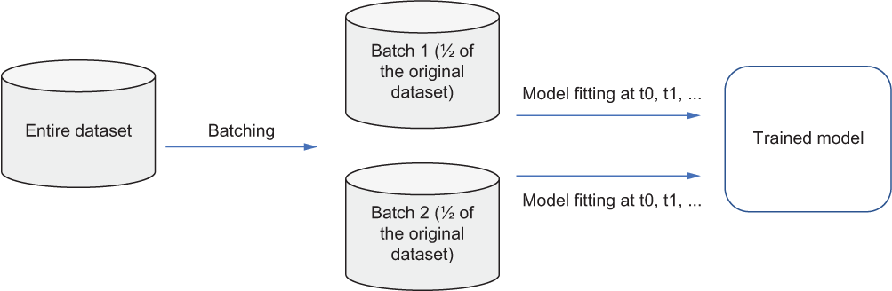
Training these types of machine learning algorithms usually involves optimizing a large set of parameters that are heavily interdependent. In fact, it can require a lot of labeled training examples to get the model close to the optimal solution. This problem is exacerbated by the stochastic nature of batch gradient descent in deep learning algorithms, in which the underlying optimization algorithm is data-hungry.
Unfortunately, the types of multidimensional data that these algorithms require, such as the data in the Fashion-MNIST dataset, may be expensive to label and take up large amounts of storage space. As a result, even though we need to feed the model lots of data, the number of samples available is generally much smaller than the number of samples that the optimization algorithm needs to reach a good-enough solution. There may be enough information in these training samples, but the gradient descent algorithm takes time to extract it.
Fortunately, we can compensate for the limited number of samples by making multiple passes over the data. This approach gives the algorithm time to converge without requiring an impractical amount of data. In other words, we can train a good-enough model that consumes the training dataset for multiple epochs.
2.5.1 The problem: Re-accessing previously used data for efficient multi-epoch model training
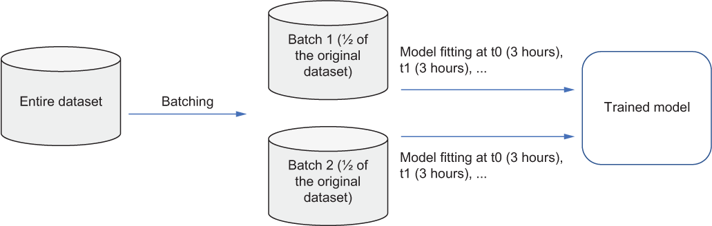
Now that we know that we can train a machine learning model for multiple epochs on the training dataset, let’s assume that we want to do this on the Fashion-MNIST dataset. If training one epoch on the entire training dataset takes 3 hours, we need to double the amount of time spent on model training if we want to train two epochs, as shown in figure 2.16. In real-world machine learning systems, an even larger number of epochs is often required, so this approach is not efficient.
2.5.2 The solution
Given the unreasonable amount of time needed to train a machine learning model for multiple epochs, is there anything we can do to speed up the process? There isn’t anything we can do to improve the process for the first epoch because that epoch is the first time that the machine learning model sees the entire set of training datasets. What about the second epoch? Can we make use of the fact that the model has already seen the entire training dataset once?
Assume that the laptop we are using to train the model has sufficient computational resources, such as memory and disk space. As soon as the machine learning model consumes each training example from the entire dataset, we can hold off recycling, instead keeping the consumed training examples in memory. In other words, we are storing a cache of the training examples in the form of in-memory representation, which could provide speed-ups when we access it again in the following training epochs.
In figure 2.17, after we finish fitting the model for the first epoch, we store a cache for both of the batches that we used for the first epoch of model training. Then we can start training the model for the second epoch by feeding the stored in-memory cache to the model directly without having to read from the data source again for future epochs.
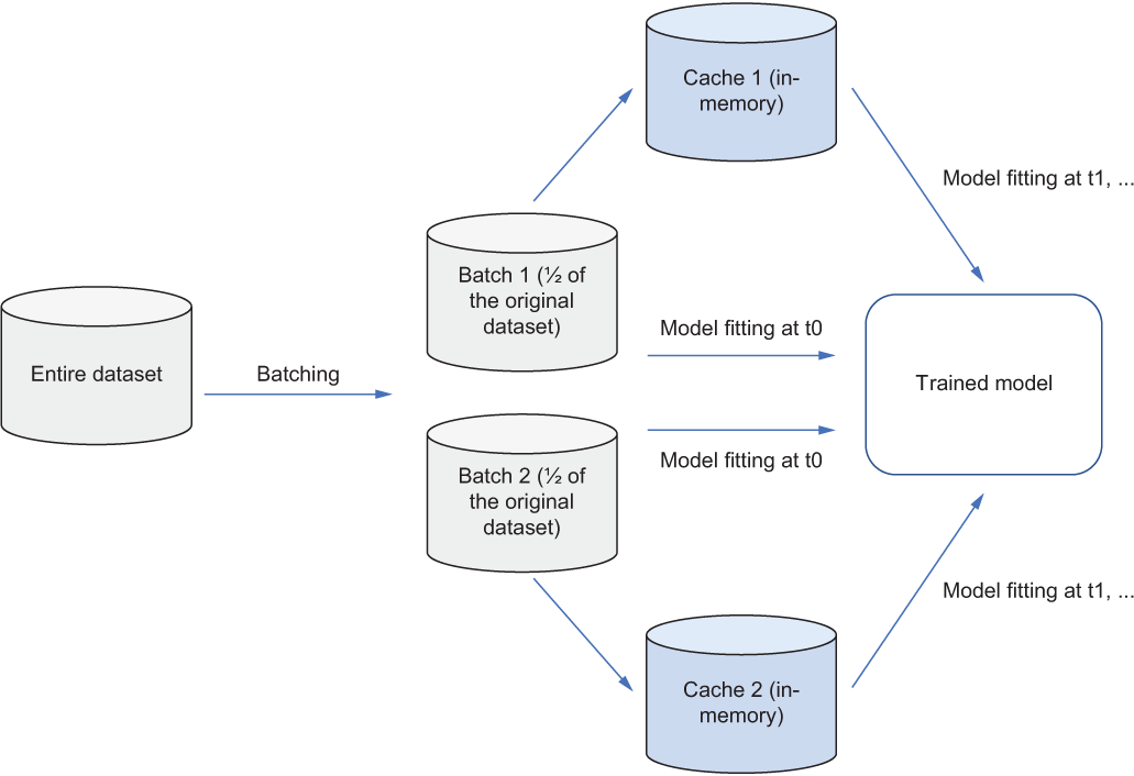
This caching pattern can be summarized as the pseudocode in the following listing. We read the next batch to train the model and then append this batch to the initialized cache during the first epoch. For the remaining epochs, we read batches from the cache and then use those batches for model training.
Listing 2.7 Pseudocode for caching
batch = read_next_batch(dataset) ❶
cache = initialize_cache(batch) ❷
while batch is not None: ❸
    model.train(batch) ❸
    cache.append(batch) ❸
    batch = read_next_batch(dataset) ❸
while current_epoch() <= total_epochs: ❹
    batch = cache.read_next_batch() ❹
    model.train(batch) ❹
❶ Reads the next batch of the dataset
❷ Initializes the cache for this batch
❸ Trains the model by iterating through the batches
❹ Trains the model for additional epochs, using the batches that were cached previously
If we have performed expensive preprocessing steps on the original dataset, we could cache the processed dataset instead of the original dataset and avoid wasting time by processing the dataset again. The pseudocode is shown in the following listing.
Listing 2.8 Pseudocode for caching with preprocessing
batch = read_next_batch(dataset)
cache = initialize_cache(preprocess(batch)) ❶
while batch is not None:
    batch = preprocess(batch)
    model.train(batch)
    cache.append(batch)
    batch = read_next_batch(dataset)
while current_epoch() <= total_epochs:
    processed_batch = cache.read_next_batch() ❷
    model.train(processed_batch) ❷
❶ Initializes the cache with the preprocessed batch
❷ Retrieves the processed batch from the cache and uses it for model training
Note that listing 2.8 is similar to listing 2.7. Two slight differences are that we initialize the cache with the preprocessed batch instead of the raw batch, as in listing 2.7, and we read the processed batch from the batch directly without having to preprocess the batch again before model training.
With the help of the caching pattern, we can greatly speed up re-access to the dataset for a model training process that involves training on the same dataset for multiple epochs. Caching can also be useful for recovering from any failures quickly; a machine learning system can easily re-access the cached dataset and continue the rest of the processes in the pipeline. We’ll apply this pattern in section 9.1.1.
2.5.3 Discussion
We have successfully used the caching pattern to store the cache in memory on each worker machine, speeding up the process of accessing previously used data for multiple epochs of model training. What if a failure happens on the worker machine? If the training process gets killed due to an out-of-memory error, for example, we would lose all the previously stored cache in memory.
To avoid losing the previously stored cache, we can write the cache to disk instead of storing it in memory and persist it as long as the model training process still needs it. This way, we can easily recover the training process by using a previously stored cache of training data on disk. Chapter 3 discusses in depth how to recover the training process or make the training process more tolerant of failure.
Storing the cache on disk is a good solution. One thing to note, however, that reading from or writing to memory is about six times faster when we are doing sequential access but about 100,000 times faster when we are doing random access rather than accessing from disk. Random-access memory (RAM) takes nanoseconds, whereas hard drive access speed is measured in milliseconds. In other words, there’s a tradeoff between storing a cache in memory and storing it on a disk due to the difference in access speedspeed. Figure 2.18 provides a diagram of model training with an on-disk cache.
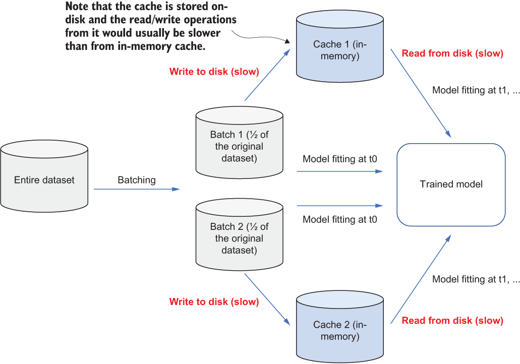
Generally speaking, storing a cache on disk is preferable if we want to build a more reliable and fault-tolerant system; storing a cache in memory is preferable when we want to have more efficient model training and data ingestion processes. An on-disk cache can be extremely useful when the machine learning system requires reading from remote databases, whereas reading from memory cache is much faster than reading from remote databases, especially when the network connection isn’t fast and stable enough.
What if the dataset gets updated and accumulated over time, as in section 2.3.3, where the data shard on each worker machine needs to be redistributed and balanced? In this case, we should take the freshness of the cache into account and update it on a schedule based on the specific application.
2.5.4 Exercises
Is caching useful for model training that requires training on the same dataset or on a different dataset for multiple epochs?
What should we store in the cache if the dataset needs to be preprocessed?
Is an on-disk cache faster to access than an in-memory cache?
2.6 Answers to exercises
Section 2.3.4
Sequentially
Yes. That’s one of the main use cases of batching.
No
Section 2.4.4
Horizontal partitioning
Locally on each worker machine
Automatic sharding, such as hash sharding
Section 2.5.4
Same dataset
We should store the preprocessed batches in the cache to avoid wasting time on preprocessing again in the following epochs.
No. Generally, an in-memory cache is faster to access.
Summary
Data ingestion is usually the beginning process of a machine learning system, responsible for monitoring any incoming data and performing necessary processing steps to prepare for model training.
The batching pattern helps handle large datasets in memory by consuming datasets in small batches.
The sharding pattern prepares extremely large datasets as smaller chunks that are located on different machines.
The caching pattern makes data fetching for multiple training rounds more efficient by caching previously accessed data that can be reused for the additional rounds of model training on the same dataset.